How to Translate Google Sheets (Cells or Full Workbooks)
 Equalang
In brief
Translate a few cells with GOOGLETRANSLATE or translate entire multi-tab Google Sheets workbooks via XLSX export while keeping numbers and formulas intact.
Keywords: translate google sheets; translate google sheets to english; translate google sheets formula; translate google sheets to spanish; googletranslate function
To translate Google Sheets, match your method to the size of your spreadsheet. If you only need to translate 10 to 100 cells into a helper column, use Google Sheets' built-in =GOOGLETRANSLATE(A2, "auto", "en") formula and paste the results as plain values. If you need to translate an entire sheet or a multi-tab workbook in place—without building mirror columns, waiting on Loading... cells, or overwriting numeric formulas—download the sheet as a Microsoft Excel (.xlsx) file (File > Download > Microsoft Excel (.xlsx)), translate the file through Equalang Document Translation, and open the translated .xlsx back in Google Sheets.
Unlike Google Docs, Google Sheets does not have a built-in Tools > Translate sheet menu that duplicates and translates a whole multi-tab spreadsheet in one click. Below are the exact steps for both workflows, depending on whether you are translating a single column or a full workbook.
Method 1: Translate 10–100 Cells with the GOOGLETRANSLATE Formula
When you have a short list of product titles, survey responses, or notes in one column and want a translation right next to them, the native =GOOGLETRANSLATE() function is the fastest tool.
The official syntax takes three arguments:
=GOOGLETRANSLATE(text, [source_language], [target_language])
text: The cell reference (such asA2) or quoted text string you want to translate.source_language(optional): A two-letter ISO language code like"es"for Spanish or"zh"for Chinese, or"auto"to let Google detect the language automatically.target_language(optional): The two-letter code for the language you want, such as"en"for English or"es"for Spanish. If omitted, it defaults to your spreadsheet's locale.
Step-by-Step: Formula + IFERROR + Paste Values Only
- Insert a helper column to the right of the column you want to translate (for example, insert column B next to column A).
- Enter the formula with an error wrapper. In cell
B2, wrapGOOGLETRANSLATEinsideIFERRORso blank cells or untranslatable symbols fall back cleanly instead of throwing#VALUE!errors:- To translate Google Sheets cells to English:
=IFERROR(GOOGLETRANSLATE(A2, "auto", "en"), A2)
- To translate Google Sheets cells to Spanish:
=IFERROR(GOOGLETRANSLATE(A2, "auto", "es"), A2)
- To translate Google Sheets cells to English:
- Fill down the column. Double-click or drag the fill handle at the bottom-right corner of cell
B2down to the end of your list. Cells will briefly showLoading...before displaying the translated text. - Lock in the text with Paste Values Only. Live
=GOOGLETRANSLATE()formulas re-evaluate when the sheet reloads. Once the translations finish loading, select your translated column, copy it (Ctrl+CorCmd+C), right-click the destination column, and choose Paste special > Values only (Ctrl+Shift+VorCmd+Shift+V). - Delete the helper column if you pasted the values back over the original text column.
Where the Formula Approach Hits a Wall
The helper-column formula works well for a few dozen rows, but it becomes awkward when you need to translate a full spreadsheet:
- Thousands of cells stall on
Loading...: Dragging=GOOGLETRANSLATE()across thousands of rows triggers slow batch evaluation and frequent timeouts. - Broken column structure: Because a formula cannot overwrite the cell it reads from, translating a 15-column table requires either inserting 15 helper columns or building a separate mirror tab.
- Mixed text, numbers, and formulas: If you drag a translation formula across a full 2D grid that includes prices, dates,
SUMtotals, orVLOOKUPreferences, the formula turns your live calculations into plain text strings.
Method 2: Translate an Entire Google Sheet or Multi-Tab Workbook via XLSX
When you need the whole spreadsheet translated in place—keeping every row, column, and calculation where it belongs—take advantage of Google Sheets' native .xlsx export and import.
By exporting to .xlsx, running the file through Equalang Document Translation, and opening it back in Google Sheets, every text cell is translated in its original position while numbers and formulas stay untouched.
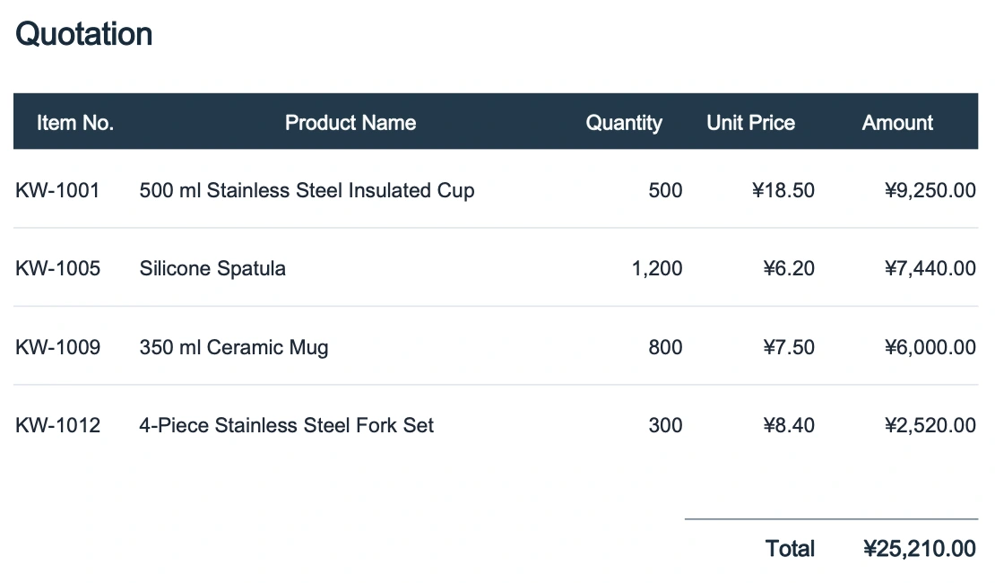
Step 1: Download Your Google Sheet as Microsoft Excel (.xlsx)
- Open your spreadsheet in Google Sheets.
- Click File > Download > Microsoft Excel (.xlsx).
- This downloads all tabs in your workbook into a single
.xlsxfile while preserving cell formatting, colors, and standard formulas.
Step 2: Upload the .xlsx File to Equalang
- Go to Equalang Document Translation and sign in.
- Upload your
.xlsxfile and choose your target language. Document translation currently covers Chinese, English, Japanese, Korean, Spanish, French and other languages, with automatic source language detection. - Start the translation and download the finished
.xlsxfile when it completes. You can also inspect the file in the online translation workspace first.
Here is what Equalang does inside your .xlsx workbook during translation:
- Numbers and formulas stay untouched: Pure numeric cells, arithmetic formulas (
SUM,AVERAGE), cross-sheet references, andVLOOKUPformulas skip the translation engine completely and are written back as-is, so totals still recalculate when you change a quantity. - Repeated strings cost once: Spreadsheets often repeat the same status labels, category names, or department codes across thousands of rows. Equalang translates and bills each identical cell text only once (see Pricing for credit rates).
- In-cell styling stays intact: Inline bold text, font colors, and line breaks inside cells carry over to the translated cells. For a deeper look at spreadsheet structure handling, see our guide on how to translate an Excel file (or if you are working with flat text exports, how to translate a CSV file).
Step 3: Open the Translated Workbook Back in Google Sheets
- In Google Sheets, click File > Import > Upload and select your translated
.xlsxfile (or drag the.xlsxinto Google Drive, right-click it, and choose Open with > Google Sheets). - Choose Replace spreadsheet (if importing into a blank sheet) or Create new spreadsheet to keep your original and translated workbooks separate.
Three Things to Check After Importing Back to Google Sheets
Even when cell positions and arithmetic formulas stay intact, spreadsheet translations have three practical boundaries worth checking before you share the sheet:
- Quoted text inside conditional formulas stays in the source language: Equalang does not rewrite formula syntax. If a cell uses a text condition like
=IF(F2="In Stock", 1, 0)or=IF(A2="Yes", B2*0.1, 0), the quoted string"In Stock"or"Yes"remains in the original language while columnForAis translated. Update the quoted condition in the formula bar to match the translated cell label so the condition evaluates properly. - Sheet tab names are not translated: To prevent breaking cross-sheet references like
='Sales_Q1'!B2:B50, worksheet tab names at the bottom of the workbook stay in the source language. Rename the tabs manually in Google Sheets if your readers need localized tab titles, and Google Sheets will automatically update your cross-sheet formula references. - Column widths and unit names: Translated text (especially when translating from Chinese or Japanese into English or Spanish) often takes up more horizontal space. Select the columns and double-click a column boundary to auto-fit widths. Also review hardware or bill-of-materials columns where manufacturer names or unit abbreviations (like
pcs) may have been localized.
Frequently Asked Questions
Does Google Sheets have a one-click "Translate sheet" button like Google Docs?
No. Google Docs has a Tools > Translate document menu that creates a translated copy of a document, but Google Sheets does not offer an equivalent one-click menu for full spreadsheets. You either use the =GOOGLETRANSLATE() cell formula for small ranges or export the workbook as .xlsx to translate all tabs in place.
How do I stop =GOOGLETRANSLATE() from saying Loading... every time I open the sheet?
Once your =GOOGLETRANSLATE() cells finish showing the translated text, select those cells, copy them (Ctrl+C or Cmd+C), and press Ctrl+Shift+V (Cmd+Shift+V on Mac) or use Edit > Paste special > Values only. This replaces the live formula with static translated text so Google Sheets stops re-fetching translations.
Will exporting a Google Sheet to .xlsx and translating it break my SUM or VLOOKUP formulas?
Standard arithmetic formulas (SUM, AVERAGE) and lookup formulas (VLOOKUP, cross-sheet references) are preserved during .xlsx export, skipped by Equalang during translation, and written back untouched. The only formulas you need to adjust manually are conditional formulas that match against a quoted text string (such as =IF(A2="Yes", ...)), where the quoted word inside the formula remains in the original language.